IGMAS+ Release v1.4.8840

Table of Contents

Overview

The new release v1.4.8840 is a significant update that enhances functionality and stability of IGMAS+. The addition of interface inversion functionality and improved import/export features, alongside the rectification of numerous bugs related to visualization, voxel cubes, and file handling, ensures a smoother and more efficient user experience. The update also brings valuable improvements in project management, user interface, and overall performance.

Highlights

Below are the main highlights from the full list of changes.

Inversion of interface geometry

In order to level up the inversion capabilities of IGMAS+, we added the new Interface Inversion plugin. With this plugin it is possible to iteratively invert (or optimize) the geometry of an interface using the misfit between the measured and calculated (at each iteration) field. The inversion (optimization) is done using the Evolution Strategy with Covariance Matrix Adaptation, or CMA-ES (Hansen and Ostermeier, 1997; Hansen, 2016; Weng, 2019), which works well demonstrates fast convergence in high-dimensional space and is able to overcome local minima of the misfit functional.

More information on the CMA-ES optimization approach is given in our recent publication:

described in our post about the 3D spring-based inversion: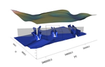

However, in the Interface Inversion plugin we do not utilize the spring-based geometry optimization concept. Instead, we adjust only the vertical coordinates of the interface vertices and perform an automatic check of the topology after each iteration.

Demonstration of interface inversion

In order to explain the interface inversion concept better, we designed a simple example with a 20km x 20km x 10km half-space model, e.g. a model with two bodies, upper and lower. In the original (reference model) the interface between the two bodies is flat and lies at 5 km depth, and in the test model the vertices of the interface is arbitrary changed:

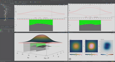
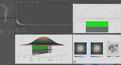
The inversion process with around 1400 generations from the initial standard deviation of 0.1 km (for interface vertices) to a stop quality threshold of 0.001 takes about 1 hour on an average laptop:

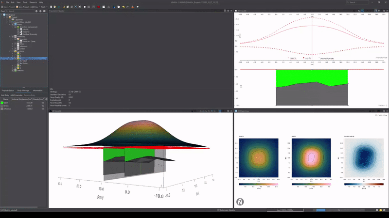
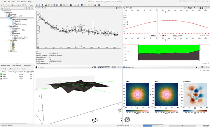
The final result shows that the original flat interface is almost perfectly reconstructed with minimal residual gravity field:

Interface inversion statistics

The Population Quality tab (top left on the previous figure) shows how the quality is changing with generations. The following statistical information is given in the Info field:

Name	Description
Strategy	Type of the evolution strategy (ES) being used
Standard Deviation	Standard deviation of depth coordinates of interface vertices compared to the previous ES generation (in m or km, depending on the project units)
Stop-Quality SD	The minimum required value of the quality to stop the ES
Evaluation(s)	Total number of evaluations of the ES
Recent quality	The minimum quality value from the recent ES generation
Non-Feasible count	Number of generations with triangle intersections

The quality value $Q$ is the standard deviation ($\sigma$) of the misfit (difference between the measured and calculated fields), normalized by the error $E$ assigned to the measured field (default is 0.2):

$$ Q_f = \sigma_f / E_f $$

In this way, the qualities of different fields can be combined to obtain the total quality:

$$ Q = Q_{f1} + Q_{f2} $$

It is possible to extract the statistical data in CSV format using the icon in the top right corner of the tab:

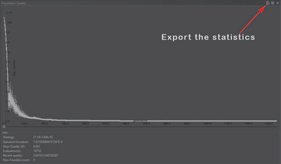
The data are extracted in columns delimited with ; in the following format (without header):

Generation Number	Standard Deviation	Quality values for the current generation
0	0.1	10.03742040705887 …
1	0.09549594023672725	10.04390540613275 …
…	…	…
1400	7.92165689475729E-4	9.908126596667E-4 …

Interface inversion workflow

Here is the minimal workflow to start the interface inversion:

• Load or create the model with at least one interface
• Load the measured data
• In the Workspace tab, right click on Interfaces and select Add Category
• Choose Inversion and click OK
  • The new Inversion entry will appear in Interfaces
• Add an interface to the Inversion category
  • Pick the desired interface and drag it to the Inversion entry
• Open interface inversion dialogue using the start icon

  

  • Interface inversion settings window will open:

    

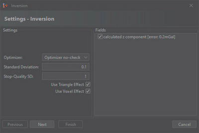
    • Select the Optimizer
      • Optimizer tri-check: enable checking if triangles in the mesh modified after each generation are intersecting (results in longer evaluation time)
      • Optimizer no-check: no checking is enabled (faster, but can result in an inconsistent mesh with intersections)
    • Adjust the Standard Deviation: the initial standard deviation of depth coordinates of interface vertices
    • Adjust the Stop-Quality SD: the threshold value of the quality
    • Select the effects to be used for the update of the calculated fields:
      • Use Triangle Effect: involve calculation of effect of the triangulated bodies
      • Use Voxel Effect: involve calculation of the effect of the voxel cubes
    • Select a desired field to use in optimization: by default all available fields are used
    • Click Next
  • Area settings window will open:

    

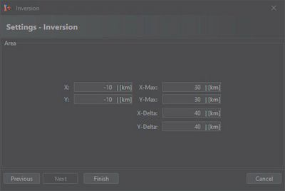
    • The default area is the area covered by stations
    • Click Finish
• Inversion process will start
  • To stop the inversion process use the stop icon

    

• Once inversion is done, the stop icon will change back to the start icon

Feel free to use the simple two-body model from our example above for testing.

• Download example model

Stability

In this release we devoted a lot of time to improvement of stability of IGMAS+.

The list of fixed problems ranges from resolution of graphical problems (various issues in the 3D, 2D and Multiple-Cutter Views, as well as rendering images in the WorldWind plugin) to file handling (loading and parsing TSURF and CSV files, loading VXO files, exporting SVG files), project management (including backward compatibility) and installation (Windows and Linux) fixes.

The most valuable improvement, however, is in the area of accuracy of potential field calculations for models that consist of both triangulated surfaces and voxel cubes.

The following inconsistency has been fixed:

Voxel Effect Algorithm	Case 1	Case 2	Case 3
Newton FFT (Multicore)	correct	wrong	wrong
Newton Masspoint (Multicore)	correct	correct	correct
Newton Masspoint (OpenCL)	correct	wrong	wrong
Prism (Multicore)	correct	correct	correct
Prism (OpenCL)	correct	wrong	wrong
Gauss quadrature (Multicore)	correct	correct	correct
Gauss quadrature (OpenCL)	correct	wrong	wrong

• Case 1: The voxel cube lies completely within the triangulated bodies.
• Case 2: There are no triangulated bodies in the model, only the voxel cube.
• Case 3: The voxel lies partially inside the triangulated bodies, partially outside.

In the release v1.4.8840 the voxel effect calculations in all cases and for all algorithms are correct.

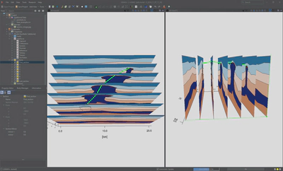
Working sections

Creating working sections has become much more convenient and intuitive:

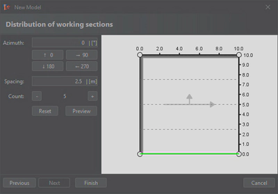
It is now easier to set up the spacing between the working sections, the overall number of sections and their orientation.

The azimuthal angle of the normal is now controlled by four direction buttons as well as the input field to an accuracy of 2 decimal places:

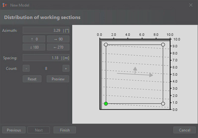
Moreover, the user can more easily define the area covered by the working sections and reset the settings if needed.

Working sections with the same orientation can also be added using the menu entry Edit ⇒ Add sections.

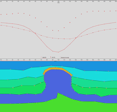
Line styles

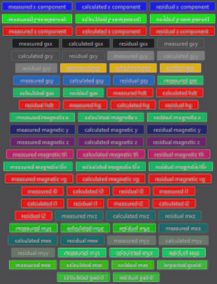
Now, by default, in the 2D and Multiple-Cutter Views user can distinguish between measured, calculated and residual fields using lines of the same color (e.g., red in case of z component), but different line styles:

Field	Line style	Example
measured	solid	━━━━━━━━━━
calculated	dashed	⁃⁃⁃⁃⁃⁃⁃⁃⁃⁃
residual	dotted	▪ ▪ ▪ ▪ ▪ ▪ ▪

For example:

The user can change the color and the line thickness by clicking on the corresponding legend entry:

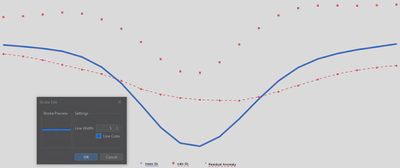
These settings are saved in the user profile and will be kept for all IGMAS+ sessions of this user.

Here is the full color pallette of default field colors:

Import of lines

In the new release, it is possible to load and visualize lines in the 3D View, in addition to point sets and bitmaps.

Line coordinates must be represented in a CSV file with columns delimited with spaces in the following format with headers:

“x0”	“y0”	“z0”	“x1”	“y1”	“z1”
6.5	2	-1.3	8.5	4	-0.87
8.5	4	-0.87	9.47	6	-1.09
9.47	6	-1.09	12	8	-0.94
12	8	-0.94	15.1	10	-1.47

Here "x0", "y0", "z0" in the header represent the 3 coordinates of the starting point of the line, while "x1", "y1", "z1" are the 3 coordinates of its end. Each data row corresponds to one line segment.

• Download sample line file

List of changes

Added

• Import of lines
• Interface inversion functionality
• Bounding box for interface inversion
• Export of quality and standard deviation values per generation after interface inversion
• Nearest neighbour interpolation for empty voxels while importing voxel cubes
• Special panel for empty voxel cells after importing a voxel cube

Changed

• Colours and line styles for fields in the 2D view
• Triangulation check message corrected to Topology check
• Misleading wording in the voxelization panel: “cubes” changed to “cells”
• Redesign of the sectioning wizard
• Title of the new model wizard
• Default header for imported CSV files

Fixed

• Incorrect 3D rendering of intersecting bitmaps with enabled transparency/alpha channel
• Graphical issue after deletion of the stations
• Issues during interface inversion
• Problem with voxel import while using grouping option
• Exception in MarchingCubesPlugin
• Problem with density geoid inversion
• Problem with missing anomaly field after loading the project
• Visualization of crossing triangles in the 2D view
• Errors in voxelization resulting in voxels with zero density
• Problem with creating a project using horizon import
• Wrong effective density value in the information tab
• Problem with SVG export from the Multiple Cutter View
• Coordinate issues while creating new project using import of horizons
• Wrong voxel visualization in 2D View when using non-square voxel cells
• Bug with re-installation of older version on top of the newer
• Incorrect calculation of the border effect in case when the density of the model units is not given in t/m3
• Wrong name for the standard deviation in linear parameter inversion, voxel effect
• Error in distance unit conversion while loading voxel cubes
• Incorrect vertical placement of loaded bitmaps in the Multiple Cutter View
• Not updating body volume values after automatic correction of polygon orientation
• Problem while loading horizons with identical points as CSV files
• Incorrect parsing of headers of certain TSURF GOCAD files
• New body added to a model is not assigned the existing properties
• Installer is not creating shortcuts on Linux
• Wrong calculation of voxel effect when combined with triangulation
• Bug while rendering images in the WorldWind plugin
• Effective density in information tab is shown even outside of the voxel cube
• Wrong application of default voxel function to the bodies deactivated during the voxel import
• Voxel cube is not visible in the 2D View
• Wrong assignment of the voxel cells to bodies after geometry changes
• Image files with names containing space are not reloaded with project
• Problem with visualization and calculation after loading voxel cubes of susceptibility type
• Problem with loading projects created with earlier versions
• Wrong effective density in information tab while voxel factor is not equal to 1

Download

Download this release either from the repository or from the archive.

• Download the installer for release v1.4.8840

Citation

Please cite this version as:

References

• Hansen, N., and A. Ostermeier (1997). Convergence properties of evolution strategies with the derandomized covariance matrix adaptation: The (μ=μ−l,λ)-CMA-ES. Proceedings of the Fifth European Congress on Intelligent Techniques and Soft Computing, 650–654.
• Hansen, N. (2016). The CMA evolution strategy: A tutorial. arXiv preprint. DOI: 10.48550/arXiv.1604.00772.
• Weng, L. (2019). Evolution strategies, https://lilianweng.github.io/posts/2019-09-05-evolution-strategies